Task Rank Is Imprinted in the Input Layer

Working draft, not yet submitted anywhere. Corpus, instruments, and this snapshot are now public, archived on Zenodo.

Abstract (draft)

Where does training leave a signature in a deep network, relative to the statistical skeleton the same architecture has at initialization? We train 1,569 bias-free ReLU MLPs at a fixed He-Gaussian specification on classification tasks whose aggregate input mean and covariance match the analytic null’s premise (0, I) exactly — as a mixture, its higher moments remain non-Gaussian, a recorded residual — and census the population against matched analytic and empirical nulls. We find an exact law: the input weight matrix of every converged net carries precisely C−1 significant dimensions — the rank of the class-mean simplex — invariant to width and class separation, verified per-net with zero exceptions, and closely tracked on real data (8.25–9.4 ≈ C−1). Deeper in the network the learned code is real but rotation-hidden: same-task twins overlap only at chance in raw eigenbases at every depth, yet carry the same code up to a fitted rotation. And the random weight bulk that censuses often score as structure is functionally inert: accuracy moves under 1% while weight decay sweeps the bulk across three orders of magnitude of scale. We map where these signatures break — a class-count frontier logarithmic in width and compute, whose capacity-proportional form we pre-registered and falsified — and release the corpus with full per-net training provenance, the audited instruments, and the negative results. Throughout, the contribution is the reading itself: a trained network treated as a measured deviation from the analytically computable null its architecture defines at initialization.

1. Motivation

We investigate whether structure measured from weights alone can predict where learned representation will appear once inference starts. Given a trained net and the statistical skeleton its architecture has at initialization, which properties of the activation geometry (location, rank, persistence, identity) are already fixed by the weights, and which require input to materialize?

This work bridges two research lines.

Moment-propagation estimators for random-weight networks provide an analytic null: what a given architecture looks like with zero learned structure, computable from the specification, no forward passes. The concrete instance is the ARC White-Box Estimation Challenge [ARC Challenge 2026; backbone paper Wu et al. 2026], which scores exactly this skill on random MLPs under a FLOP budget — a tractable proxy for the Alignment Research Center’s larger estimation agenda: analytic prediction of network behavior in regimes where sampling is uninformative (rare and tail behaviors, anomaly detection). That agenda ultimately concerns trained models, and the challenge write-up’s “toward non-random networks” section names the missing object — a population of trained networks with shared statistics — and defers it as future work. Meanwhile, label-free structure mining in trained models finds low-dimensional, depth-persistent activation geometry, but with no matched untrained population to diff against it cannot say which parts are learned rather than architectural.

We built 1,569 trained nets at the challenge’s exact Phase-1 architecture, matched to the analytic null in everything except training. The thesis this population supports: training leaves a low-rank, analytically measurable signature in the weights that predicts where representation will form, before inference runs (§4.1–4.3). The remaining results map that thesis’s boundaries: the signature fixes where structure lives but not which directions carry it — coordinate identity is rotation-hidden and needs an anchor (§4.4); quantitative spectrum prediction holds only under population-fitted corrections (§4.7); and the class-count frontier and the inert weight bulk locate where the instruments themselves stop reading (§4.5, §4.6). What follows downstream (§5.3) is implication, not additional contribution.

2. The corpus

Architecture: ARC Phase-1 spec — square bias-free ReLU stacks, He-Gaussian N(0, 2/fan_in) init, ReLU after every layer; a bias-free linear head outside the censused stack carries the readout (its necessity and its gradient side-effects are themselves catalogued: a frozen-column no-head variant provides an in-net guaranteed-null control).
Tasks: Gaussian mixtures analytically whitened so the aggregate input has mean 0 and covariance I exactly (as a mixture, its higher moments remain non-Gaussian — the residual mismatch with the null’s Gaussianity assumption is recorded per net; class count C ∈ {2..64} and separation are dials; Bayes accuracy computed exactly per task), plus whitened MNIST and Fashion-MNIST (784→d seeded projection + ZCA; real higher moments, matched second moments).
Axes: width {64, 128, 256, 512}, depth {8..64}, budget {20k, 60k, 200k}, weight decay {0..1.0}, learning rate arms, two readout modes, 16–32 seeds per configuration; 1,569 nets, 69 families, every net with full provenance (task, hyperparameters, seeds, outcome label vs exact Bayes, trajectory).
Infrastructure: batched-stack trainer (32 nets/process, init bit-identical to the sequential reference, 64 s/net on a laptop GPU); upload-verify-prune corpus lifecycle with HF as system of record.

3. Instruments

Eight instruments, each audited (§8), each running from committed code (census/, null_baseline/; vendored provenance in PROVENANCE.md). The first two read weights only — zero forward passes; the next three read activations on controlled inputs; the last three are correction, tracking, and wild-model machinery.

3.1 Weight census (census/manifold_detector.py; vendored from our earlier activation-structure tooling — the label-free structure-mining line of §1 — with source and adaptations recorded in PROVENANCE.md). Per-layer eigenspectrum census of the weight matrices themselves. For a layer’s uncentered second-moment spectrum {λᵢ}, the Marchenko–Pastur bulk edge is λ₊ = σ²(1 + √γ)², γ the matrix aspect ratio [Marchenko & Pastur 1967]; significant dims = #{λᵢ > λ₊}. Two floors are always reported: the fixed analytic floor σ² = 2/fan_in, exact because the He init scheme is known by construction (the matched-corpus instrument, §4.1); and a robust estimate σ̂² = median(λ)/m(γ), m the MP median factor, for models whose init is unknown (§5.4). Alongside: effective dimension via participation ratio PR = (Σλᵢ)²/Σλᵢ², and a bulk_regime flag (intact/depleted) that gates which reading is meaningful — under strong weight decay the bulk falls below any floor and MP counting is undefined (§4.6).

3.2 Analytic state trajectory — the q-clock (null_baseline/state_trajectory.py + the vendored Hermite moment chain [ARC Challenge 2026; Wu et al. 2026]). Propagates (μ, Σ) = (0, I) through the trained weights with the uncorrected k=2 Hermite chain — an analytic computation on the weights, no data. Per-layer descriptors: q = PR(Σ_pre)/w (the rank-collapse clock: 1 isotropic → 0 collapsed), ā/āsd (mean/std of the per-neuron ReLU operating point μ/σ), r̄ (mean |ρ| off-diagonal correlation). The null is a band: the same descriptors over 50 fresh He inits per architecture; trained readings are z-scores against that band (§4.2).

3.3 Activation census with init-anchored floor (census/run_activation_census.py). The eigenspectrum census on post-ReLU activations, under matched task and pure-noise inputs (identical mean and covariance by construction, §4.3). The floor is anchored to init: per layer, the init net’s maximum activation-eigenvalue fraction is the threshold, and significant_dims_anchored counts trained eigenvalue fractions exceeding it — a matched empirical exceedance null. Validity is regime-bound and recorded per layer: clean where init activations are diffuse (early layers), inverted where init has rank-collapsed below trained (depth) — there the trained/init effective-dim ratio is the statistic (§4.3).

3.4 Directional consistency (census/directional_consistency.py). Does training move the input layer in the same direction across seeds, and toward the task? Uᵢ = top-(C−1) left singular vectors of ΔW₀ = W₀ᵗʳᵃⁱⁿᵉᵈ − W₀ⁱⁿⁱᵗ; subspace overlap(A, B) = ‖AᵀB‖²_F / k — mean cos² of the principal angles — against the exactly-known task subspace T = orthonormal basis of the centered class means (a GMM-construction privilege), and pairwise across seeds. Isotropic chance is k/d (§4.1, §4.5).

3.5 Eigenspace overlap, raw and Procrustes-recovered (census/eigenspace_overlap.py, census/procrustes_overlap.py). Per layer: top-k eigenvectors of each net’s activation covariance on a shared input sample; pairwise overlap ‖UᵢᵀUⱼ‖²_F / k against k/d chance — the raw (coordinate-bound) reading. The recovered variant splits the shared sample into fit/test halves, fits the orthogonal Procrustes map R = UVᵀ from SVD(A_fitᵀB_fit) [Schönemann 1966] on the fit half only, and measures overlap between test-half eigenbases after the map — an estimate of how much code is shared up to an orthogonal transformation (§4.4). Orthogonal is doing real work in that sentence: the fit has no scaling or translation freedom, so recovered overlap cannot come from amplitude matching; and R = UVᵀ ranges over the full orthogonal group, reflections included — “rotation” in this paper always means this orthogonal class.

3.6 Population-refit state-keyed stabilizer (null_baseline/refit_trained.py + vendored chain_state_keyed.py [ARC Challenge 2026]). Repairs §3.2’s chain on trained weights. The chain’s 16 correction slots become functions of measured state rather than layer index: c_j = θ_j · g(state), the basis g built from (q, ā, āsd, r̄) — 128 parameters; two indicator dims [is_first, is_last] extend it to 160 and fix the edges. θ is fit by DAgger-style iteration [Ross et al. 2011]: roll trajectories with the current θ, regress residual-to-truth at every layer, repeat. Polish iterations are accepted or rejected on the validation population’s final-layer error — the validation set therefore participates in model selection; the C=50 population is reserved untouched for transfer evaluation (§4.7).

3.7 Transport-corrected feature tracking (census/feature_tracker.py; vendored from the same structure-mining tooling as §3.1, provenance in PROVENANCE.md). Matches activation eigenfeatures layer-to-layer, raw and after linear transport through the layer map. In this corpus it is chiefly a calibrated negative result: chain-level feature continuity in plain MLPs is not recoverable under raw or transported matching — only through data-fitted rotations (§4.4) — which bounds what tracking can claim elsewhere.

3.8 Entry-shuffled empirical null for wild models (census/wild_census.py). For each wild weight matrix, an entry-shuffled copy — identical marginal entry distribution and scale, structure destroyed — is censused as that matrix’s own null, requiring no knowledge of the init scheme. Validated on first contact: the wild models’ own reinitializations read 0–1 significant dims, spectrally indistinguishable from the shuffle (§5.4); the shuffle null also caught an orientation artifact on first use.

4. Results

4.1 The input-rank law (exact)

Terms: “significant dims” counts eigenvalues of a weight matrix’s uncentered Gram above the Marchenko–Pastur (MP) bulk edge at the He init variance 2/fan_in — the analytic bound on how large a purely random eigenvalue can be at this shape; anything above it is structure the null cannot produce.

Under the fixed analytic floor, L0 significant dims = C−1. This is exact per-net for all 240 converged nets across C ∈ {2..32} and separations 1.5–6.0 (including a task with Bayes accuracy 0.505); reads 8.25–9.4 on real data (closely tracking C−1 but not exact per-net); confirmed independently by the scaled floor at C ≥ 15. Partially-trained nets show the count still accreting after accuracy plateaus — at every failure boundary we probed (class-count wall, width and depth optimization failures) the input layer keeps learning the task geometry (task-subspace alignment 0.38–0.89 of converged levels at chance accuracy). Learning proceeds at the input edge even when the pipe fails.

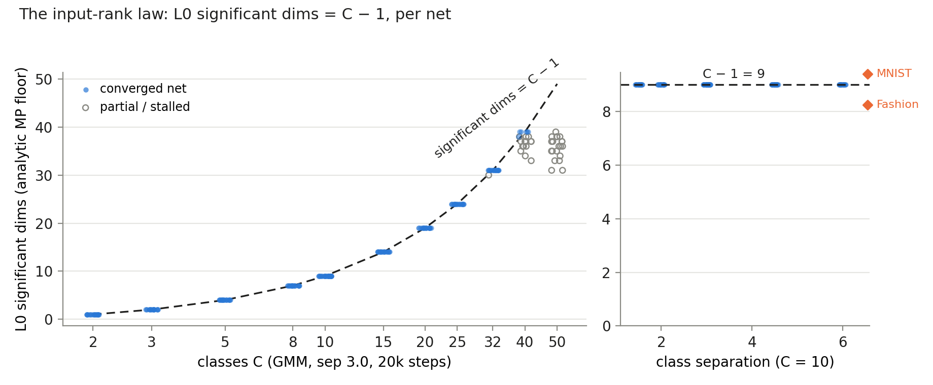Fig 1 — the input-rank law Figure 1. The input-rank law. Left: per-net L0 significant dims under the analytic MP floor vs class count; every converged net (filled) sits on C−1 exactly; partial learners (open) scatter below while still accreting. Right: the law is invariant to class separation 1.5–6.0 at C=10; whitened MNIST and Fashion-MNIST read 9.4 and 8.25 ≈ C−1.

4.2 The analytically-propagated terminal rank is task-driven, two-sided

Terms: the “q-clock” is q(L) = PR/w, the participation ratio (effective dimension) of the analytically propagated pre-activation covariance at layer L, normalized by width; “null band” is the per-architecture q(L) distribution over freshly initialized nets.

Random nets’ propagated rank decays to a depth-driven fixed point. Trained nets’ analytically-propagated terminal rank tracks the task code instead: +3 to +4σ above the architecture’s null band for mid-C, below it for small-C/easy tasks and MNIST, at-band for uncommitted partial learners; strongest in narrow nets (+11σ at w=64), inverted at shallow depth (−7.5σ at d=8). One law, signed by the task’s rank demand relative to the architecture’s fixed point. Caveat: the clock runs the uncorrected analytic chain, which carries significant spectrum error on trained weights (§4.7) — but it is used here as a matched comparison, the same chain on trained and random weights against the same null band, not as a spectrum predictor, and its terminal reading is corroborated activation-side by §4.3’s deep inversion.

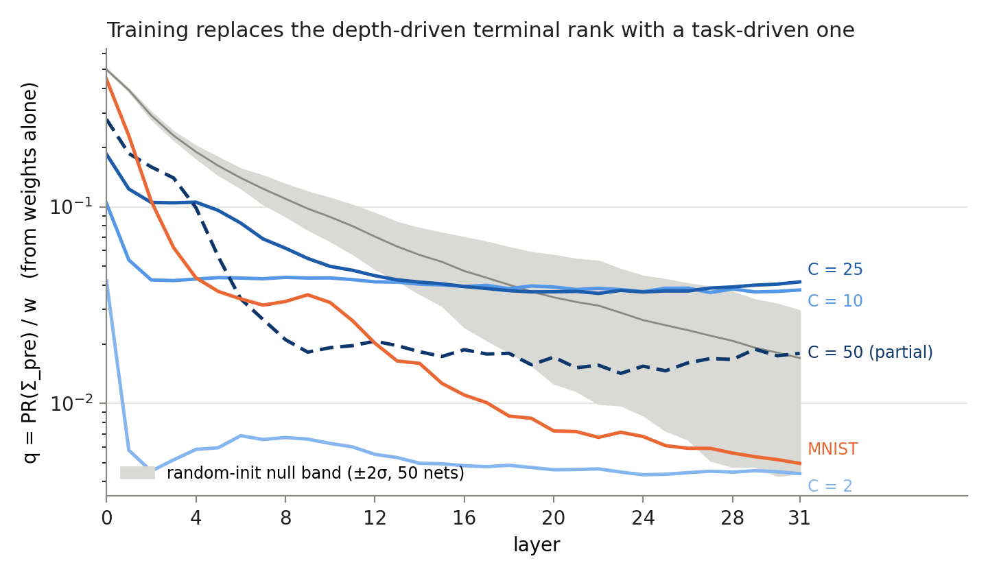Fig 2 — the q-clock Figure 2. Family-median q-clock trajectories (w=256, d=32) against the 50-net random-init null band. Mid-C tasks arrest above the band’s fixed point; C=2 and MNIST need less rank than depth alone would leave and exit below it; the uncommitted C=50 partial learners ride the band — the clock measures committed structure. Computed from weights alone.

4.3 Noise-driven activations carry the structure; task input sharpens it

The GMM construction makes this comparison confound-free: task input and pure N(0, I) noise match in mean and covariance exactly, so any activation difference is higher-moment.

Trained-weight activations under pure noise already carry the qualitative structure signature; task input tightens it modestly. Under the init-anchored exceedance floor, the early-activation rank law mirrors the weight law: L1 anchored significant dims read C−1 to C for C ≤ 20 (2.0/3.0/5.0/7.4/9.0/14.0/19.0) and collapse with the wall (13.8 at C=40). The C=25/32 readings (20.0/19.6) sit at the instrument’s stored top-20 eigenvalue cap and are right-censored — lower bounds, not ceiling measurements (the C ≤ 20 law and the C=40 collapse are below the cap and unaffected; §4.5’s mid-net code ceiling is measured by effective dimension, computed from the full spectrum, and is also unaffected). At mid/deep layers the exceedance count reads ≈ 0 everywhere — and that is itself the finding: init activations at depth are more rank-collapsed than trained ones, so trained structure at depth is not “spikier than init” but less collapsed than init — the activation-side view of §4.2’s arrest. The valid deep statistic is the trained/init effective-dim ratio, not any exceedance count (the anchored floor is clean exactly where init is diffuse and inverts where init has collapsed; both counts plus the anchor are recorded per layer).

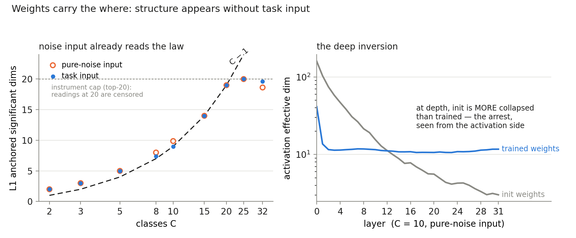Fig 3 — weights carry the where Figure 3. Left: L1 anchored significant dims vs C under pure-noise (open) and task (filled) input — the noise reading already sits on the C−1 law; task input changes it only marginally. The C=25/32 points sit at the instrument’s top-20 cap (dotted line) and are right-censored. Right: activation effective dimension vs depth for the same weights before and after training (noise input): init activations collapse below trained ones past mid-depth, so at depth trained structure is “less collapsed than init,” not “spikier than init.”

Same-task twins: L0 input-coordinate subspaces overlap 0.86–0.93 (init controls exactly at isotropic chance); raw hidden-space eigenbases at or near k/d chance at every depth; Procrustes-recovered overlap 0.99 early / 0.90 deep for twins against 0.38 for init controls; a cross-task condition reads 0.67, but it was measured under noise input rather than task input, so it is not input-matched with the twin condition — a bound, not a clean task-similarity grading. Chain-level feature tracking fails in plain MLPs under both raw and linearly-transported matching — continuity of the code is recoverable only through data-fitted rotations. Consequence for representational-convergence claims: convergence is real, rotation-hidden, and training-dependent (twins ≫ init controls); an input-matched cross-task rerun is needed before calling it task-graded. Metrics must be rotation-invariant or input-anchored.

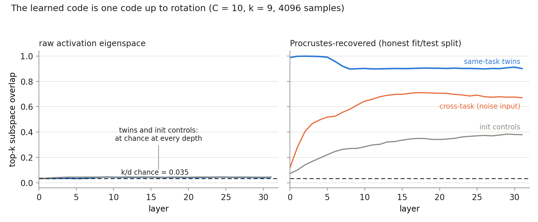Fig 4 — rotation-hidden code Figure 4. The same nets, two views. Left: raw activation-eigenspace overlap between same-task twins is indistinguishable from init controls and from k/d chance at every depth. Right: a fitted orthogonal Procrustes map (honest fit/test split) recovers 0.99 early / 0.90 deep for twins against 0.38 for init controls. The cross-task series (0.67) was measured under noise input and is not input-matched with the twin condition.

4.5 The class-count wall: pre-registered, falsified, then resolved as a logarithmic compute frontier

Terms: C₅₀ is the class count at which half the seeds converge; the “ceiling” is the mid-net activation code’s saturating effective dimension (~14 at w=256 for every C ≥ 25, converged or not).

Convergence fraction vs C at fixed budget is a sharp logistic transition at every width (logistic width ~1.5–2.2 classes; seed variance ×10 at the crossing; Bayes gap linear in C below it). We pre-registered C₅₀(w) = 2.7 × ceiling(w) — proportionality between the wall and the mid-net activation-code ceiling — and falsified it: the constant held at w=128/256 (2.54/2.53) and failed at w=64 (ratio 3.5). The resolution, from per-width lr-tuned sweeps, is that the wall is not capacity-proportional at all but a compute frontier, consistent with logarithmic growth in both width and budget over the tested range (four widths, three budgets — the data bound the shape, they do not identify it): C₅₀ = 27.8 / 32.3 / 36.2 / 38.8 at w = 64/128/256/512 (~+3.7 classes per width doubling), sliding ~+10 classes per tripling of steps (w=512, C=48: 0% → 88% converged at 3× budget). The ceiling grows comparably slowly in width (8.1/11.6/14.3), which is why the falsified proportionality appeared to hold at two widths. Ten-times budget arms show the slide continuing: crossings reach ≈ 61 (w=512) and ≈ 50 (w=256) at 200k steps — tasks unreachable at 3× budget converge at 10× — with mildly diminishing log-returns (+10 then +4 classes per budget tripling at w=256) hinting at, but not demonstrating, saturation beyond the tested decade. Every “hard boundary” we encountered at fixed hyperparameters — a w=512 stall, a depth-48/64 trainability frontier — dissolved under lr and budget scaling (d=64: from total stall to 14/16 converged), while in every failure family the input layer’s task-subspace alignment kept accreting at chance-level accuracy. Fixed-hyperparameter trainability boundaries must not be read as architectural limits.

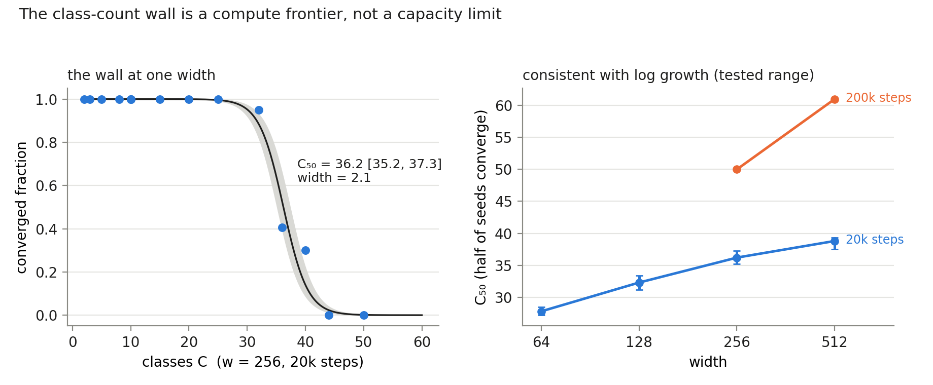Fig 5 — the wall Figure 5. Left: convergence fraction vs C at w=256/20k steps, with the committed logistic fit and bootstrap band. Right: the crossing C₅₀ vs width at 20k steps (≈ +3.7 classes per width doubling) and at 200k steps — the frontier slides with budget (no hard asymptote within 10×) and with width, nothing like proportional to capacity.

4.6 The random bulk is functionally inert

Weight decay sweeps the bulk from 1.0× to 0.000× of its He scale while accuracy moves < 0.008 — same function, same performance, completely different weight statistics. The census’s fixed floor fails abruptly at ~0.6–1.2 nats of decay while the depletion itself is smooth. In the depleted regime rank metrics, not MP counts, are the structure measure (the robust estimator provably breaks there — documented, not patched over).

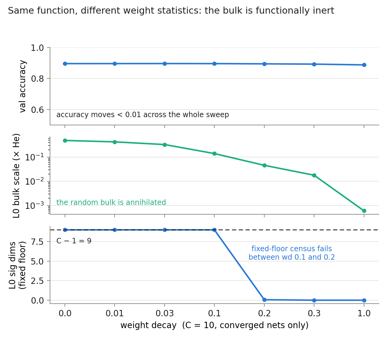Fig 6 — the bulk is inert Figure 6. The weight-decay sweep at C=10, converged nets only. Accuracy is flat (top) while the L0 random bulk is swept across three orders of magnitude of scale (middle); the fixed-floor census reads C−1 exactly until the bulk crosses the floor between wd 0.1 and 0.2, then reads zero while the structure demonstrably remains (bottom).

4.7 Quantitative skeleton prediction needs population-fitted corrections

A companion random-ensemble measurement (published separately as analytic_vs_sampling/ in our public replication of the challenge estimator [ARC Challenge 2026]) grounds the baseline: the uncorrected chain’s error is depth-flat once the state trajectory saturates (constant to <2% across d=24→48 at w=256, 48 nets/cell) and beats FLOP-matched Monte Carlo at a crossover depth that rises monotonically with width — the analytic skeleton is a stable object to correct against at any depth. On trained weights the picture changes: the k=2 mean-field chain predicts random-net activation spectra to 3–7% through 32 layers but degrades to 80%+ by L16 on trained weights. A state-keyed correction (ARC’s machinery, 160 params with edge indicators) refit on the trained population repairs the bulk 7–12× on the validation population, fixes the edges, and — fit on mixed converged+partial populations — serves both regimes. Two honesty notes: the same validation population gated polish acceptance (one scalar per iteration — a small selection pressure, but these are validation numbers, not untouched held-out estimates), and the untouched out-of-population read is the C=50 transfer set, where the refit is mixed and worse than uncorrected in some layers — the correction is population-bound. A 16-parameter constant-coefficient rung captures only ~1.4× (no hidden dominant scalar; the state-keying is load-bearing).

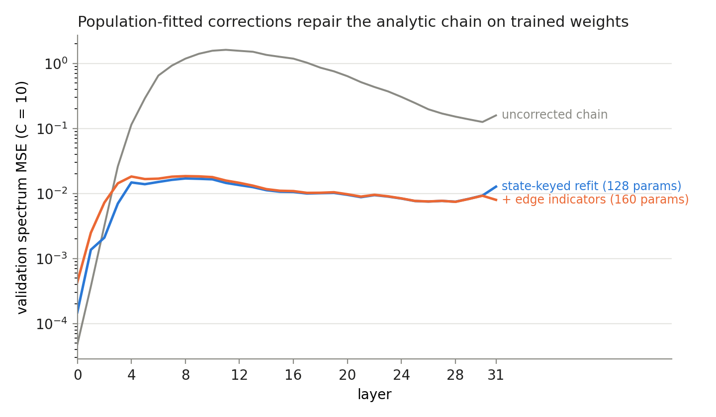Fig 7 — population-fitted corrections Figure 7. Per-layer spectrum error on the validation population (C=10) — which also gated polish acceptance: validation numbers, not untouched held-out. The uncorrected chain degrades by 80%+ mid-depth on trained weights; the state-keyed refit repairs the bulk ~7–12×; edge indicator dims fix the L0/L1 harm at zero bulk cost.

5. Discussion

5.1 The answer

One thesis, two measured boundaries. The thesis: location, rank, and persistence of activation structure are weight-determined. The input layer holds the task’s class geometry as an exact integer (§4.1); analytic propagation of the weights — zero forward passes — predicts the terminal rank of the activation code (§4.2); and trained weights driven by pure noise already produce the full qualitative structure signature, which task input tightens but does not create (§4.3). To first order, a trained net’s activation geometry is a property of its weights that inference reveals rather than creates.

First boundary: the identity of the learned code is real and shared across same-task nets, but only up to rotation (§4.4): raw hidden-space eigenbases overlap at chance at every depth while Procrustes-recovered overlap reads 0.90–0.99 for twins against 0.38 for init controls. So where structure lives is predictable from weights; which directions carry it is not even well-posed without an anchor — the input coordinates, or a fitted rotation.

Second boundary: the analytic chain predicts random-net spectra to a few percent through 32 layers but degrades to 80%+ on trained weights; a 160-parameter state-keyed correction refit on the trained population repairs the bulk ~7–12× on validation — and fails on populations from other training regimes (§4.7). No trained-network estimator comes for free; a population-specific one costs ~10² parameters, a modest matched population, a validation gate, and an untouched transfer check.

The durable contribution is the lens rather than any single number: a trained network read as a measured deviation from the analytically computable null its architecture defines. The corpus and the instrument catalog exist to make that reading exact.

5.2 Reading weights versus running the model

Inference is the end product, so we delineate precisely what can be known before a model runs. The instruments operate at three levels of access:

Weights alone, analytically (§3.1, §3.2; results §4.1, §4.2): no data, no execution. Cost is set by the specification, and the null is clean — the init distribution is known (matched corpora) or estimable from the matrix itself (§3.8).
Weights executed on structureless input (§3.3; §4.3): mechanically inference, epistemically still a weights reading — the input carries no task information, so whatever structure appears is attributable to the weights.
Weights executed on task input (§4.3, §4.4): inference proper. Every reading is now a property of the composition (weights ∘ input distribution); attributing structure to learning requires an input-matched control, which this corpus has by construction and wild models never grant.

The findings ladder onto the levels exactly: location, rank, and persistence of structure are readable at level 1; the full qualitative signature appears at level 2; level 3 adds sharpening and the coordinate realization. Across the statistics we measured, nothing appeared at level 3 whose location was not already fixed at level 1.

Each direction of reading also has a demonstrated blind spot, and they are complementary. Weight statistics are not sufficient for function: §4.6’s nets compute the same function at the same accuracy across three orders of magnitude of bulk scale. Inference readings in raw coordinates are not sufficient for identity: §4.4’s twins compute the same code while their raw (pre-Procrustes) eigenbases overlap only at chance. An audit that reads only weights can misjudge amplitude; an audit that reads only raw activations can miss identity entirely. The instrument pairing is the design, not a redundancy.

The two sides are bridged, and the bridge is itself a result: the q-clock is a prediction about inference computed without inference — conditional on the null’s input premise (mean-0, covariance-I input) — and its terminal rank matches the activation-side arrest measured under noise input (§4.2 ↔︎ §4.3). That faithfulness is what makes weight-side reading operationally useful — a model can be checked against its architecture’s null from the weights file alone, before deployment, without choosing an input distribution, and without being permitted or able to run it.

The four distinctions this section leans on — weight-encoded, execution-required, coordinate-dependent, basis-invariant — are stated operationally throughout. Why training produces invariants with exactly this structure is deliberately left open: this paper’s job is the cartography, not the theory of it.

5.3 Implications

Nothing in this section is a contribution of this paper; these are the places the thesis and its boundaries land.

For analytic estimation on real models

The ARC White-Box Estimation Challenge scores analytic prediction on random nets as a tractable proxy for the estimation problems that matter in reality — rare and tail behaviors, anomaly detection, properties of models in regimes where sampling cannot reach. Those problems live on trained models. This corpus is the controlled step between the two. Three results carry over:

The random-weight chain’s best trained-network role is the null, not the predictor. Every training signature in this paper is a measured deviation from the analytic skeleton (§4.1, §4.2, §4.6), computable from a weights file at specification cost. That is directly usable for anomaly detection: does this net deviate from its architecture’s null the way its claimed training says it should?
Corrections are cheap and population-bound (§4.7): ~10² parameters and a modest matched population suffice, and the failure mode on out-of-regime populations (partial learners) is detectable by validation gating and transfer checks, not silent.
Regime flags are mandatory instrumentation. Every instrument we fielded has a validity boundary that training economics can cross: the weight-decay knee (§4.6), the anchored floor’s inversion at depth (§4.3), the scaled estimator’s break in the depleted regime. What transfers is the paired null — fixed analytic where the init is known, entry-shuffled where it is not (§3.8) — plus a per-matrix flag saying which regime the reading came from.

For weight-space auditing and representational convergence

For weight-only model auditing: task-relevant rank is readable from weights alone, but amplitude is not learning (§4.6) — an auditor that scores spectral mass measures optimizer hygiene, and the structure measure must switch from MP counts to rank metrics once the bulk is depleted. For the representational-convergence literature: convergence across same-task models is real, training-dependent, and strictly rotation-hidden (§4.4) — cross-model comparisons made in raw coordinates at depth measure nothing, and metrics must be rotation-invariant or input-anchored to see the shared code at all. Whether models in the wild show the same signature — chance-exact raw overlap with rotation-recoverable, task-graded identity — is measurable with the same paired instruments, and is where this result asks to be tested next.

5.4 Outlook: wild models

While the above results rely on a matched corpus, preliminary tests indicate these instruments transfer to wild models. First contact with pythia-70m/160m MLP blocks (no init anchor, so scaled floor plus entry-shuffled nulls, §3.8) read per-matrix profiles of 3–111 significant dims against 0–12 for the shuffled nulls, and the models’ own reinitializations read 0–1 dims everywhere — spectrally indistinguishable from the shuffle, which validates entry-shuffling as an init-free baseline. The validity rules learned on the controlled corpus (orientation, regime flags, null choice) transferred without modification and caught one artifact on first use. The wild-model study itself — with its own controls and a pre-registered prediction of what the census should read given each model’s claimed training — is the next paper, not a result of this one.

Analytic propagation on random networks. The signal-propagation / mean-field line [Poole et al. 2016; Schoenholz et al. 2017] studies random deep nets in expectation over both weights and inputs, and the NNGP/NTK line [Neal 1996; Lee et al. 2018; Jacot et al. 2018] takes the infinite-width limit. The regime here is different and less studied: one finite network with its actual weights, statistics over random inputs — the setting formalized by the heuristic-arguments program [Christiano et al. 2022] and operationalized by the ARC White-Box Estimation Challenge and its backbone paper [Wu et al. 2026], with rare-behavior estimation as the motivating application [Wu & Hilton 2024]. We inherit that machinery unchanged and invert its role: on trained networks the propagated skeleton is the null, and deviation from it is the measurement (§4.2, §4.7).

Training signatures in weight matrices. The closest antecedent to the weight census is Thamm, Staats & Rosenow [2022], who compare trained-network weight spectra against random-matrix predictions and find the bulk still conforming to Marchenko–Pastur after training, with learned information confined to the largest singular values — RMT comparison as a way to locate learning. Martin & Mahoney read training signatures in wild models’ spectra — heavy-tailed self-regularization, quality prediction with no access to data [Martin & Mahoney 2021; Martin, Peng & Mahoney 2021]. The Neural Feature Ansatz [Radhakrishnan et al. 2024] supplies the mechanism by which task structure enters weight Grams: WᵀW tracks the average gradient outer product. The matched corpus adds to all three what their settings cannot supply: an exact analytic floor (σ² = 2/fan_in known by construction, no self-calibration), a population in which the deviation is an integer measured per net — the C−1 law — and a functional test: sweeping the bulk across three orders of magnitude at fixed accuracy shows the random remainder is inert, so spectral amplitude tracks optimizer economics, not learning (§4.6). The wd knee locates where amplitude-based reading breaks — a validity boundary the diagnostic settings inherit.

Simplex geometry and neural collapse. Neural collapse [Papyan et al. 2020] finds last-layer features of converged classifiers collapsing to the C−1-dimensional simplex ETF — an output-side, activation-space, terminal-phase phenomenon — and has since been traced into intermediate layers [Rangamani et al. 2023; Parker et al. 2023], where collapsed layers carry low-rank weights. Relatedly, SGD with weight decay provably biases weight rank down [Galanti et al. 2022; Zangrando et al. 2024]. The input-rank law (§4.1) is the input-edge, weight-space counterpart: the class-mean simplex rank imprints in W₀ under the analytic floor — and it accretes before convergence, at chance-level accuracy (§4.1, §4.5), so simplex geometry at the input edge is not a terminal-phase effect. §4.6 gives the low-rank-bias line a measurement it implies but has not run: the decayed bulk is functionally inert, and the census floor fails at a locatable knee while the structure persists.

Representational similarity and convergence. The alignment literature [Li et al. 2016; Raghu et al. 2017 (SVCCA); Kornblith et al. 2019 (CKA)] and the Platonic Representation Hypothesis [Huh et al. 2024] argue trained representations converge; permutation/rotation symmetry work [Ainsworth et al. 2023] explains why raw coordinates cannot show it. Our controlled twin population sharpens both claims into a measurement (§4.4): with task, data, architecture, and init distribution all matched, raw eigenspace overlap sits at chance (exact at shallow layers; a small depth elevation is shared by init controls, so it is not training signal), while a fitted rotation recovers 0.90–0.99 for twins against 0.38 for init controls — convergence is real, strictly rotation-hidden, and training-dependent. Anchor-based “relative representations” [Moschella et al. 2023] operationalize the same prescription from the engineering side: comparisons made relative to fixed anchor samples are invariant to latent isometries, which is §4.4’s input-anchored reading as a design principle.

Model zoos and weight-space learning. Populations of trained nets exist as datasets for meta-learning — model zoos [Schürholt et al. 2022], accuracy prediction from weights [Unterthiner et al. 2020]. Those populations vary hyperparameters to cover behavior space; ours is constructed to match an analytic null (single init scheme, bias-free, aggregate input distribution equal to the null’s premise, exact per-task Bayes), which is what makes deviation-from-null a defined quantity. To our knowledge no prior population was built against a computable null.

7. Limitations

Single architecture family (plain ReLU stacks); GMM tasks are linearly separable by construction (real-data families partially address this); the Bayes proxy mislabels real-data outcomes; the wall is characterized as a compute frontier (§4.5) but its mechanism — and its relation to the code ceiling — is unresolved; correction scope across optimizers and objectives is unmeasured (AdamW wild models are first-contact only, §5.4). The next falsifiable step mirrors this paper’s method: pre-register what the census should read on a wild model given its claimed training, then check.

8. Audit trail

An external adversarial audit of the first findings digest found two findings wrong as stated (stale pilot numbers; a self-calibrating floor) and five oversold precisions; all were rewritten from current data, the falsified pre-registration is reported as falsified, and every instrument’s failure modes are documented in-repo. A recurring statistical lesson enforced throughout: per-net error quantities in this regime are heavy-tailed (both Monte-Carlo and analytic-closure errors; max/median 10–22× at depth), so small-sample mean-based comparisons flip sign under reseeding — medians with bootstrap intervals are the reporting standard, with per-net records committed. The corpus, instruments, per-net provenance, and audit note ship with the paper.

9. References

(Every entry verified 2026-08-18 against arXiv metadata, publisher pages, or a previously audited internal citation ledger — none written from memory. In-text keys: Wu et al. 2026 is Wilson Wu (challenge backbone); Wu & Hilton 2024 is Gabriel Wu.)

ARC White-Box Estimation Challenge (2026). Competition organized by the Alignment Research Center on AIcrowd. https://www.aicrowd.com/challenges/arc-white-box-estimation-challenge-2026. Warm-up June 10–17; Phase 1 June 18–July 31; Phase 2 August 1–September 19,
1. Accessed 2026-08-18; archived at https://web.archive.org/web/20260818152858/https://www.aicrowd.com/challenges/arc-white-box-estimation-challenge-2026.
Ainsworth, S. K., Hayase, J., & Srinivasa, S. (2023). Git Re-Basin: Merging Models modulo Permutation Symmetries. ICLR 2023 (oral). arXiv:2209.04836.
Christiano, P., Neyman, E., & Xu, M. (2022). Formalizing the presumption of independence. arXiv:2211.06738.
Galanti, T., Siegel, Z. S., Gupte, A., & Poggio, T. (2022). SGD and Weight Decay Secretly Minimize the Rank of Your Neural Network. arXiv:2206.05794.
Huh, M., Cheung, B., Wang, T., & Isola, P. (2024). Position: The Platonic Representation Hypothesis. ICML 2024. arXiv:2405.07987.
Jacot, A., Gabriel, F., & Hongler, C. (2018). Neural Tangent Kernel: Convergence and Generalization in Neural Networks. NeurIPS 31, 8571–8580. arXiv:1806.07572.
Kornblith, S., Norouzi, M., Lee, H., & Hinton, G. (2019). Similarity of Neural Network Representations Revisited. ICML 2019, PMLR 97, 3519–3529.
Lee, J., Bahri, Y., Novak, R., Schoenholz, S. S., Pennington, J., & Sohl-Dickstein, J. (2018). Deep Neural Networks as Gaussian Processes. ICLR 2018. arXiv:1711.00165.
Li, Y., Yosinski, J., Clune, J., Lipson, H., & Hopcroft, J. (2016). Convergent Learning: Do different neural networks learn the same representations? ICLR 2016. arXiv:1511.07543.
Marchenko, V. A., & Pastur, L. A. (1967). Distribution of eigenvalues for some sets of random matrices. Matematicheskii Sbornik 72(114)(4), 507–536. English translation: Mathematics of the USSR-Sbornik 1(4), 457–483.
Martin, C. H., & Mahoney, M. W. (2021). Implicit Self-Regularization in Deep Neural Networks: Evidence from Random Matrix Theory and Implications for Learning. Journal of Machine Learning Research 22(165), 1–73. arXiv:1810.01075.
Martin, C. H., Peng, T. S., & Mahoney, M. W. (2021). Predicting trends in the quality of state-of-the-art neural networks without access to training or testing data. Nature Communications 12, 4122. arXiv:2002.06716.
Moschella, L., Maiorca, V., Fumero, M., Norelli, A., Locatello, F., & Rodolà, E. (2023). Relative representations enable zero-shot latent space communication. ICLR 2023 (oral). arXiv:2209.15430.
Neal, R. M. (1996). Bayesian Learning for Neural Networks. Lecture Notes in Statistics 118. Springer.
Papyan, V., Han, X. Y., & Donoho, D. L. (2020). Prevalence of Neural Collapse during the terminal phase of deep learning training. PNAS 117(40), 24652–24663. arXiv:2008.08186.
Parker, L., Onal, E., Stengel, A., & Intrater, J. (2023). Neural Collapse in the Intermediate Hidden Layers of Classification Neural Networks. arXiv:2308.02760.
Poole, B., Lahiri, S., Raghu, M., Sohl-Dickstein, J., & Ganguli, S. (2016). Exponential expressivity in deep neural networks through transient chaos. NeurIPS 29 (NIPS 2016). arXiv:1606.05340.
Radhakrishnan, A., Beaglehole, D., Pandit, P., & Belkin, M. (2024). Mechanism of feature learning in deep fully connected networks and kernel machines that recursively learn features. arXiv:2212.13881. Published as “Mechanism for feature learning in neural networks and backpropagation-free machine learning models,” Science (2024), doi:10.1126/science.adi5639.
Raghu, M., Gilmer, J., Yosinski, J., & Sohl-Dickstein, J. (2017). SVCCA: Singular Vector Canonical Correlation Analysis for Deep Learning Dynamics and Interpretability. NeurIPS 30 (NIPS 2017). arXiv:1706.05806.
Rangamani, A., Lindegaard, M., Galanti, T., & Poggio, T. A. (2023). Feature learning in deep classifiers through Intermediate Neural Collapse. ICML 2023, PMLR 202, 28729–28745.
Ross, S., Gordon, G. J., & Bagnell, J. A. (2011). A Reduction of Imitation Learning and Structured Prediction to No-Regret Online Learning. AISTATS
1. arXiv:1011.0686.
Schoenholz, S. S., Gilmer, J., Ganguli, S., & Sohl-Dickstein, J. (2017). Deep Information Propagation. ICLR 2017. arXiv:1611.01232.
Schönemann, P. H. (1966). A generalized solution of the orthogonal Procrustes problem. Psychometrika 31(1), 1–10.
Schürholt, K., Taskiran, D., Knyazev, B., Giró-i-Nieto, X., & Borth, D. (2022). Model Zoos: A Dataset of Diverse Populations of Neural Network Models. NeurIPS 2022, Datasets and Benchmarks Track. arXiv:2209.14764.
Thamm, M., Staats, M., & Rosenow, B. (2022). Random matrix analysis of deep neural network weight matrices. Physical Review E 106, 054124. arXiv:2203.14661.
Unterthiner, T., Keysers, D., Gelly, S., Bousquet, O., & Tolstikhin, I. (2020). Predicting Neural Network Accuracy from Weights. arXiv:2002.11448.
Wu, G., & Hilton, J. (2024). Estimating the Probabilities of Rare Outputs in Language Models. arXiv:2410.13211.
Wu, W., Lecomte, V., Winer, M., Robinson, G., Hilton, J., & Christiano, P. (2026). Estimating the expected output of wide random MLPs more efficiently than sampling. arXiv:2605.05179.
Zangrando, E., Deidda, P., Brugiapaglia, S., Guglielmi, N., & Tudisco, F. (2024). Provable Emergence of Deep Neural Collapse and Low-Rank Bias in L²-Regularized Nonlinear Networks. arXiv:2402.03991.